Background
Spatially resolved transcriptomics (SRT) has made it possible to quantify gene expressions within specific locations of a tissue section. Some of the SRT platforms can offer cellular or sub-cellular resolution, while others usually provide the sum of expressions for a few neighbouring cells within a spot. To know more about SRT platforms, please check out one of my blogposts on this topic here.
After deriving the data from SRT platforms, it has to be put through some preprocessing pipelines depending on the platform used, which will then generate a count matrix. Then, low-quality signals, such as poorly captured genes and cells/spots need to be removed. To know more about this quality control step, please check out my blogpost on this here.
The gene expression data or the count data is impacted not only by biology but also by technical factors such as differences in library sizes. So, it has to be normalized. Ideally, normalization should get rid of the unintended library size effects while preserving the biological effects. In fact, the success of downstream analyses such as domain identification and spatially variable gene detection among others, heavily depends on that of the normalization step.
In most cases, single-cell-specific normalization methods are still being used to normalize SRT data. However, library sizes can vary across spatial regions. If this factor is not taken into account during normalization, region-specific library size biases may make it hard to extract biologically relevant signals from the data. Figure 1 shows how library sizes can vary depending on spatial regions.
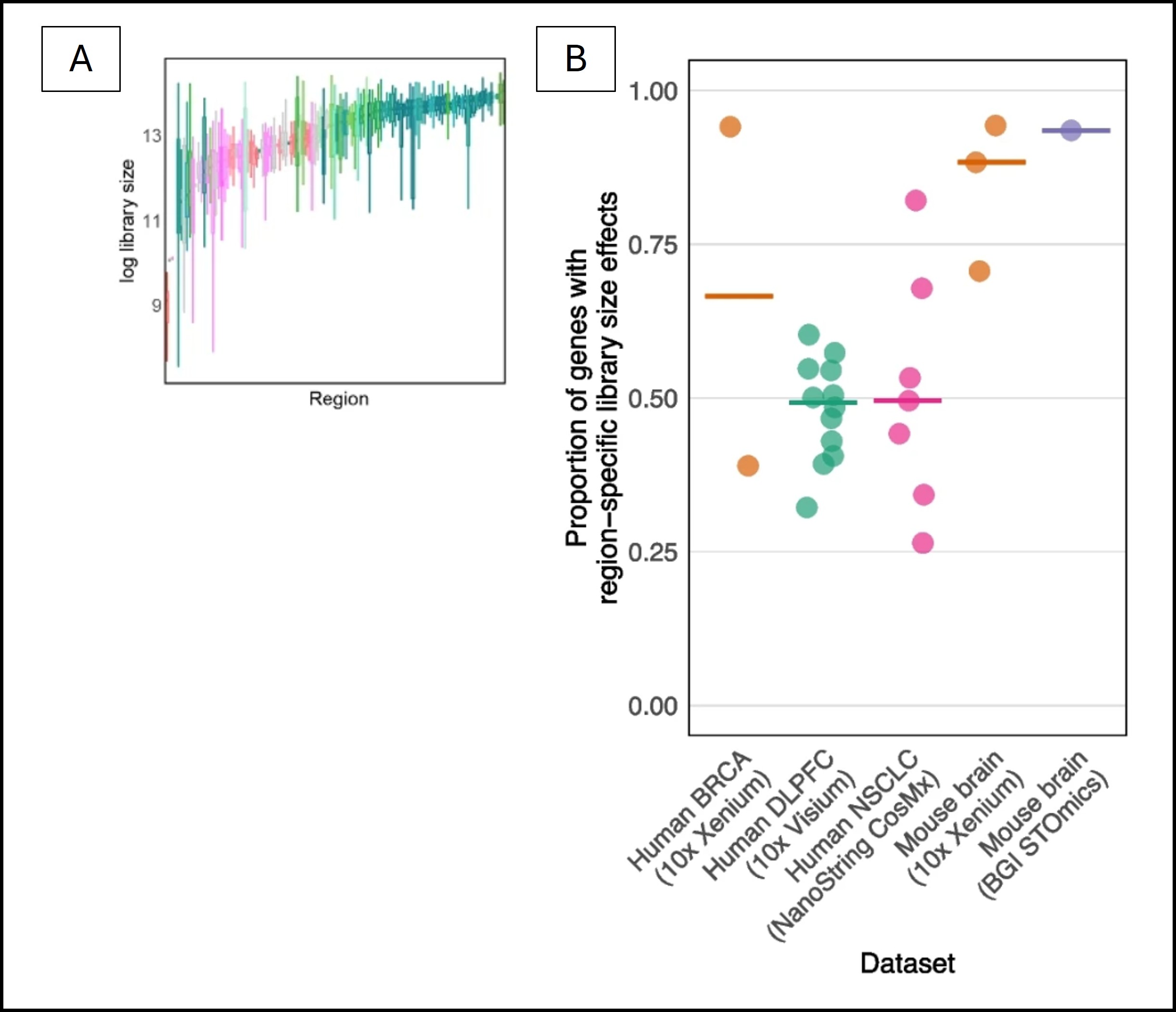
Figure 1: Library sizes may show region-specific biases. (A) log-transformed library sizes vary across the spatial regions. (B) Depending on the SRT platform, different proportions of genes may demonstrate region-spcific library size effects. Both of these figures were adapted from the article being explored in this post.
Last year (2025), the first spatially-aware normalization method SpaNorm was published, which can be implemented using a Bioconductor package. This blogpost will walk the reader through this method.
SpaNorm: how it works
The innovation
SpaNorm offers three innovations -
It computes spatially smooth functions using thin plate splines to derive gene- and cell/spot-specific factors instead of relying on global factors,
It optimally decomposes spatial variation into two spatially smooth variations - one of them is associated with library sizes, whereas the other one is independent of library sizes and thus assumed to be biologically relevant,
It adjusts the data using various adjustment approaches including percentile-invariant adjusted counts.
The core concept
The following schematic diagram (Figure 2) helps visualize the core concept of SpaNorm -
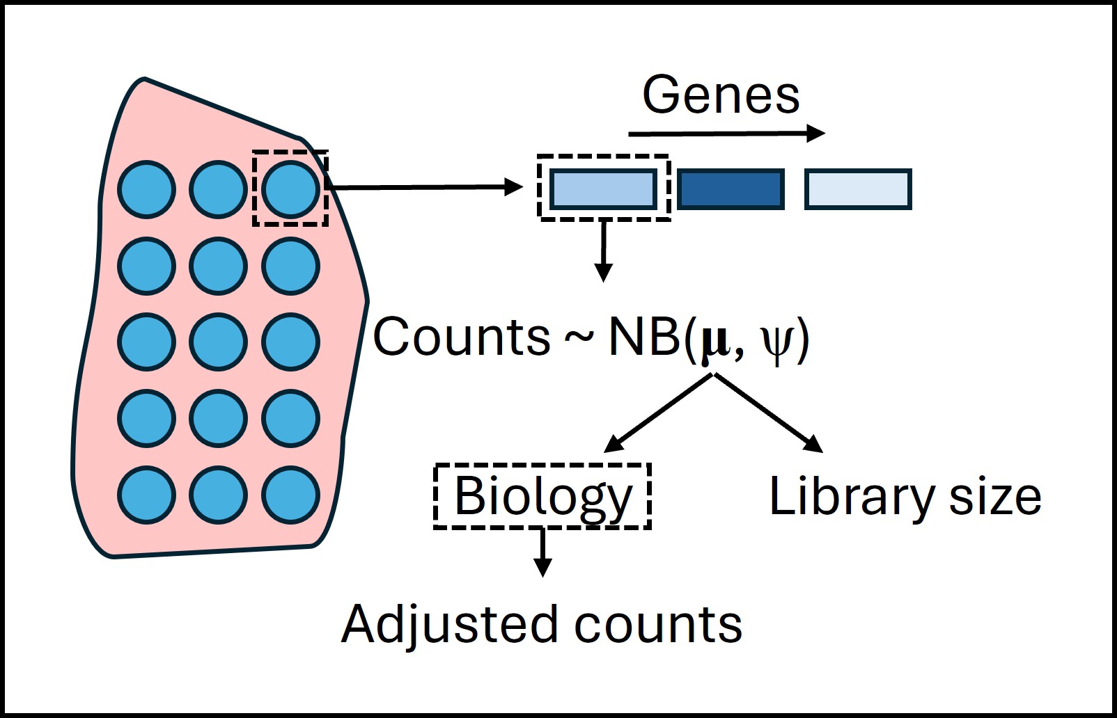
Figure 2: A schematic diagram showing the core concept of SpaNorm. The blue circles represent spots or cells overlaid on the tissue (red) to show where they are coming from. SpaNorm assumes that the counts for each gene in each spot follow a binomial distribution with cell/spot and gene-specific mean (\(𝛍_{gc}\)), along with gene-specific dispersion (\(𝛙_g\)) parameters. It then assumes that the biological and library size effects influence \(𝛍_{gc}\) through a log-linear model. So, after fitting the model, there will be a term for biology and another one for library size. The estimated biological effects can then be used to derive adjusted counts, which can be transformed to get the normalized counts.
The algorithm
The math/stat behind it
Let’s now take a step-by-step journey through the algorithm, starting with the equation for the aforementioned log-linear model -
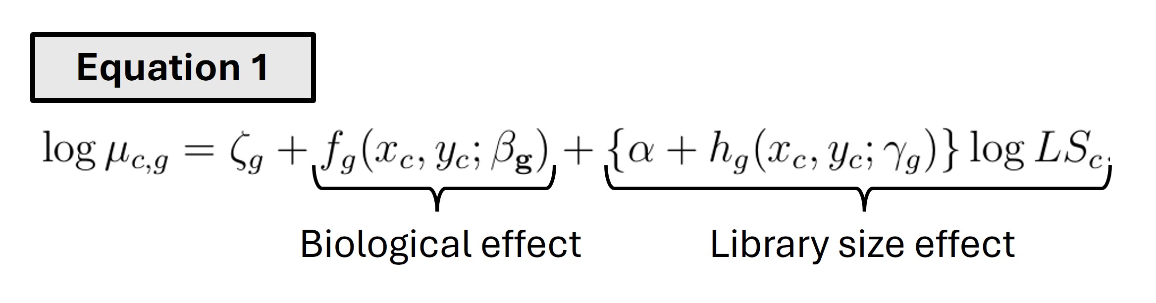
Here, \(LS_c\) is the library size for spot/cell c. 𝝰 and \(𝛄_g\) are the global and gene-specific library size effects, respectively. Similarly, \(𝛃_g\) is gene-specific biological effect. Both the biological and library size effects have a function each - namely, \(f_g\) and \(h_g\). Let’s try to understand what they do -
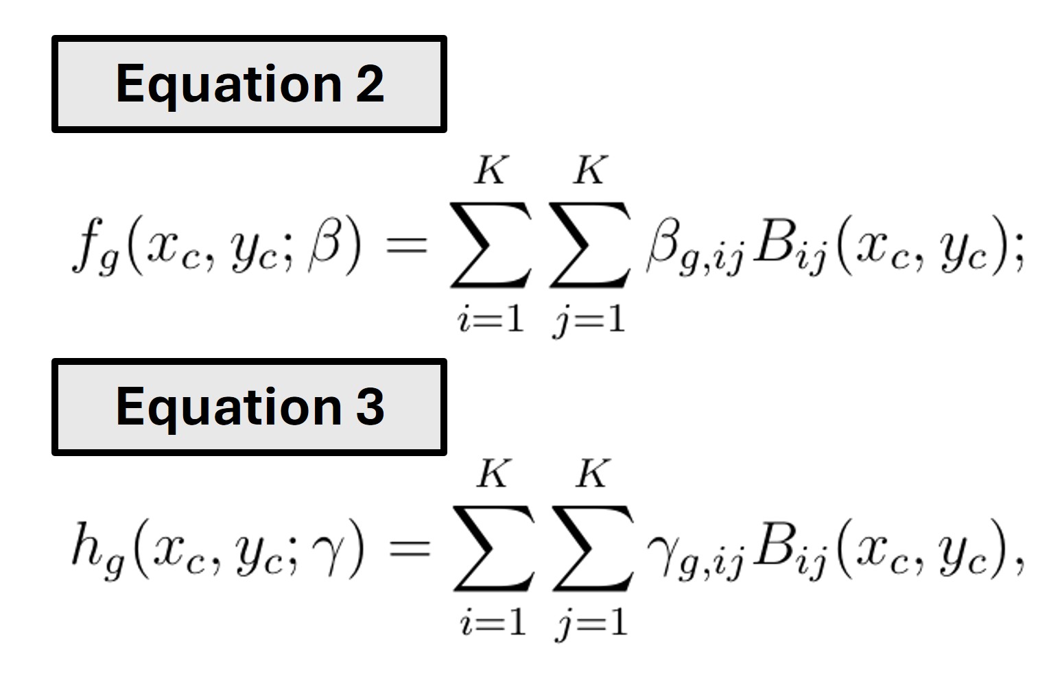
In equations 2 and 3, (\(x_c\), \(y_c\)) are spatial coordinates of spot/cell c. \(f_g\) and \(h_g\) are two-dimensional gene-specific spatially smooth functions constructed using 2D splines with K degree of freedom. B indicates B-splines basis functions.
It all may seem a bit complicated. Just think of it this way. The tissue slide is two-dimensional. Both of these dimensions will impact the gene expression values, which can be thought of as sheet or surface with bumps and depressions at various locations. SpaNorm assumes there two such surfaces - one comprises both biology and library size effects and the other one is devoid of the library size effect. The goal is to find what these two surfaces look like.
To fit the model, equation 1 is rewritten as -
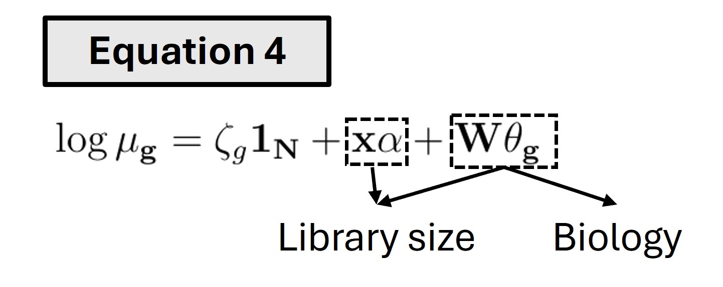
Here, X is a vector of log-transformed library sizes. W is a matrix of basis functions applied to spatial coordinates. Both \(B_{ij}\)(\(x_c\), \(y_c\)) and \(B_{ij}\)(\(x_c\), \(y_c\))\(LogLS_c\) values are included in W. \(𝛉_g\) is a vector of gene-specific biological and library size effects. As can be seen in equation 4, the W\(𝛉_g\) term can be decomposed into two parts. One part will inform biology and the other part, along with X𝝰, will form library size effect.
Estimating the parameters of interest
The goal is now to find the global library size effect 𝝰, gene-specific dispersion \(𝛙_g\), intercept \(𝛇_g\) and \(𝛉_g\). These parameters are estimated using a double-loop iterative reweighted least squares (IRLS) algorithm. IRLS is widely used to fit generalized linear models (GLMs). To know more about it, please read this blogpost on Medium.
The workflow used in SpaNorm is delineated below -
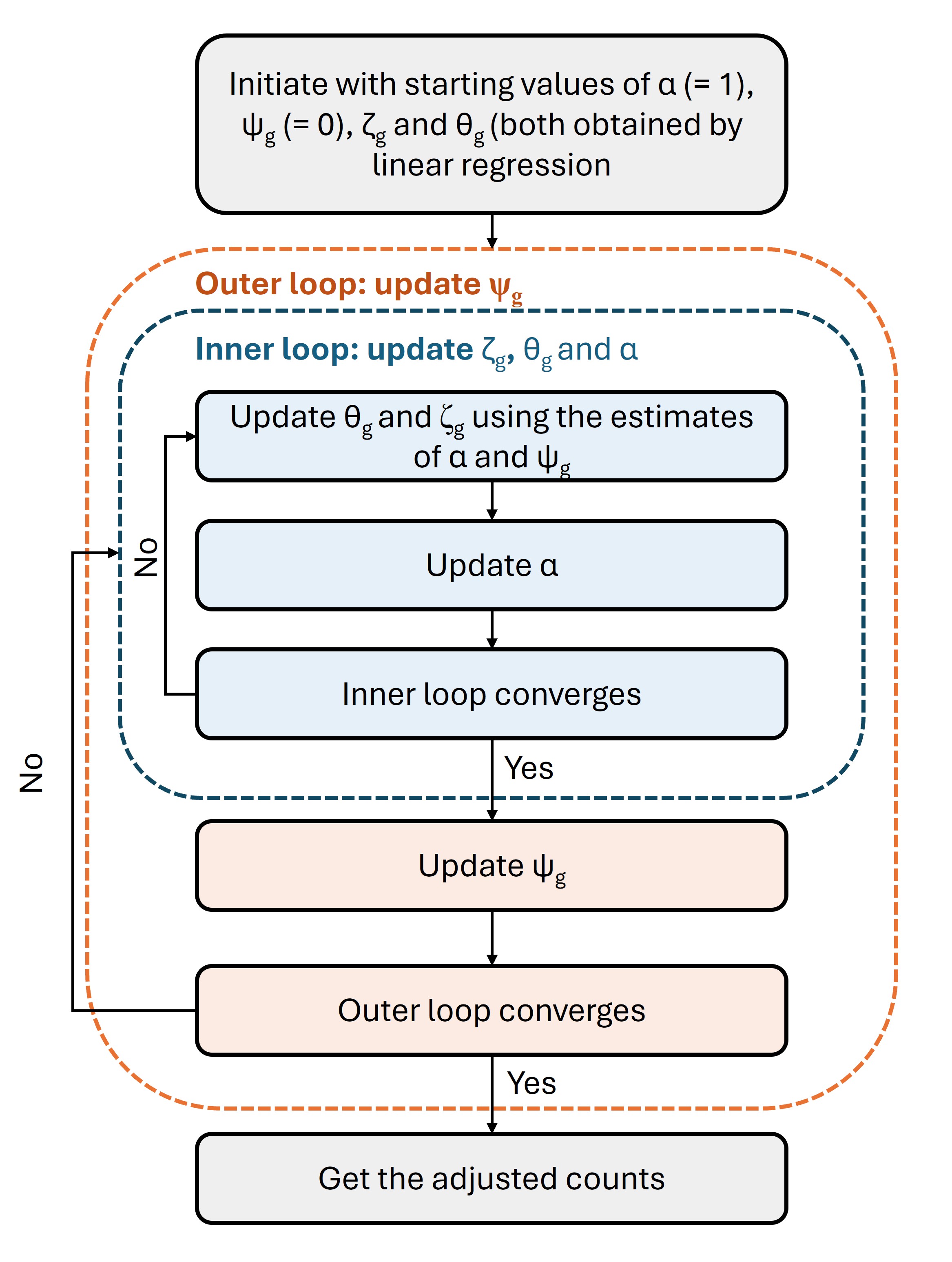
Figure 3: The algorithm to estimate the global and gene-specific parameters and get the adjusted data
First, the values of 𝝰 and \(𝛙_g\) are set to 1 and 0, respectively. Then, linear regression is performed using the log(count/library_size + 1) values as response variables to get the initial estimate of \(𝛇_g\). The regression coefficients for W are considered as the starting value of \(𝛉_g\).
Next, in the inner loop of the double loop IRLS process, \(𝛉_g\) and \(𝛇_g\) are first updated using the current estimates of 𝝰 and \(𝛙_g\). The estimate of 𝝰 is then updated. If the inner loop converges, the outer loop is started. Otherwise, the inner loop is repeated (that is why, it is called iterative).
Once the inner loop converges, \(𝛙_g\) is updated in the outer loop. If this loop does not converge, the inner loop is restarted with the latest parameters. When convergence occurs in the both loops, adjusted data can be derived.
Getting the adjusted counts
The estimated parameters are used to obtain the percentile-invariant adjusted counts (PACs) using the following equation -
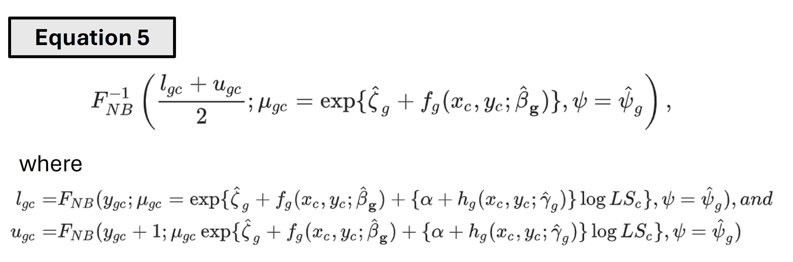
The \(F_{NB}\) functions are cumulative density functions of negative binomial distributions with library size effects. Since count data is discrete, for any given raw count, that count and the count next to it (count + 1) are both considered. Then the quantile of the negative binomial distribution without the library size effect is considered to be the PAC. The normalized counts can simply be calculated as log(PAC + 1). Other adjustment methods are also available through the SpaNorm package.
Concluding remarks
Library sizes in SRT data can display region-specificity. If this bias is not taken into account during the normalization step, the quality of downstream analyses may be compromised. SpaNorm is the first spatailly aware normalization method for SRT data. Although the original article only focused on library sizes as sources of technical variations, effects of other unwanted covariates can also be estimated and removed by this method. Besides, the authors showed that the method works well with both spot-based and single-cell-based SRT approaches and out-performs existing normalization methods on downstream tasks like spatially variable gene detection and spatial domain identification.